🏃♀️ Navigating Big O: A Journey from O(1) to O(n!)

Welcome back to the continuation of our series on Big O! If this is your first blog entry and you're interested in this topic (often out of necessity due to interviews, but interested nonetheless to improve...) you've probably asked yourself some of these questions:
❓ How do software engineers or programmers, however, you prefer to call them, evaluate the efficiency of algorithms? How do they decide which is the best method to solve a specific problem? The answer often lies in a type of mathematical analysis known as Big O Notation.
Big O is an essential component in computer science that allows professionals to compare the efficiency of different algorithms in terms of runtime and resources consumed. Thanks to Big O, we can predict how an algorithm will behave as the volume of data increases. This is crucial for making informed and objective decisions about which algorithm to use in a given situation.
First, I invite you to review the previous posts in the series to have more information about the topic:
In this post, we'll embark on a journey through the different types of Big O Notation, from constant time (O(1)) to factorial time (O(n!)), exploring how each impacts the performance of our algorithms. Additionally, we'll provide code examples, pros and cons, as well as some practical applications of each. And to help you visualize how the runtime varies based on the data input, we'll also include descriptive charts of each type. So if you're ready to unravel the mysteries of Big O Notation, let's get started 🏁!
Constant Time - O(1)
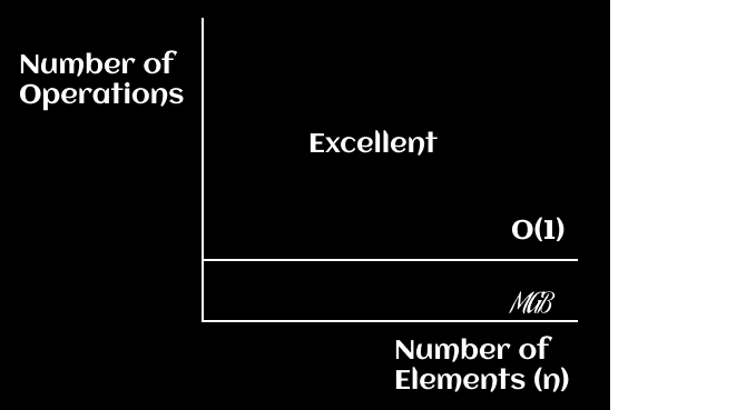
Constant time, denoted as O(1), describes an algorithm whose execution time is independent of the amount of data. Imagine you have a book and you want to see the first page. It doesn't matter if the book has 100 or 1,000 pages, it will always take you the same amount of time to open it and see the first page. This is a good example of a constant time in real life: the number of pages (data) in the book doesn't affect the time it takes to perform the operation (open the first page).
Here's a code-level example of a function that takes no arguments and always returns the same result. It doesn't depend on any input and therefore is a constant time algorithm O(1).
const sayHello = () => 'Hello world';
Common Use Cases
A good example of constant time is accessing a specific element in an array by its index. Regardless of the size of the array, the runtime to access an element by its index will always be the same.
1. If you have an array of millions of elements and you want to access the element at the index 500,000, you can do it directly and the time it will take won't be affected by the length of the array.
const array = [1, 2, 3, 4, 5, ..., 1,000,000];

console.log(array[500000]);
2. Determining if a number is even or odd. No matter how large the number, the runtime will be the same.
const isEven = (n) => n % 2 === 0;
3. Accessing a value in an object by its key. Regardless of how many properties the object has, it always takes the same amount of time to retrieve a value if you know the key.
const user = {
  name: 'Matías',
  age: 28,
  city: 'Córdoba',
  country: 'Argentina',
  // More properties...
};

console.log(user.name);
I hope these examples help to illustrate the concept of constant time O(1) better. Remember, the key here is that the execution time does not change, no matter how much data the algorithm is handling.
Advantages and Disadvantages
Constant time algorithms are the most efficient in terms of runtime. This is ideal for operations that need to be done quickly and do not depend on the number of elements to process.
The downside, however, is that these types of algorithms are not useful for tasks that require processing or manipulating multiple data elements, such as sorting an array or searching for a specific item in an unordered list.
Diagrams
In this case, the execution time does not change with the size of the input. So if you plot this function, you simply get a horizontal line. On an x-y plane, you can graph the function f(x) = 1
Logarithmic Time - O(log n)
A logarithmic time algorithm, or O(log n), is one whose execution time is halved with each iteration of the algorithm. Imagine you're looking for a number in a phone book. Instead of starting at the first page and going through each number one by one, you open the phone book in the middle and decide whether the number you're looking for is before or after the page you opened. This process repeats until you find the number. That's essentially what a logarithmic time algorithm does.
An example of such an algorithm is binary search, which is used to find an item in an ordered list.
const binarySearch = (list, item) => {
  let low = 0;
  let high = list.length - 1;

  while (low <= high) {
    let mid = Math.floor((low + high) / 2);
    let guess = list[mid];

    if (guess === item) {
      return mid;
    }

    if (guess < item) {
      low = mid + 1;
    } else {
      high = mid - 1;
    }
  }

  return null;
}
Common Use Cases
- Binary search is often used in database applications. When searching for a specific record in a large, ordered database, binary search can quickly find the record. Likewise, binary search trees, which are data structures based on the idea of binary search, are used in many applications, including compilers and database management systems.
- Searching in a dictionary: If you're looking for a word in a physical dictionary, you wouldn't start at the first page and move forward one by one. Instead, you'd open the dictionary approximately in the middle and determine whether the word you're looking for would be before or after in the dictionary, and then repeat the process in the corresponding half.
- Number guessing: If you're playing a game where you have to guess a number between 1 and 100, and on each attempt, you're told whether your guess is too high or too low, an efficient strategy would be to start in the middle (50) and adjust your guesses upward or downward based on the clues. In this way, with each guess, you halve the range of possible numbers.
Advantages and Disadvantages
The biggest advantage of logarithmic time algorithms is their efficiency with large data sets. As the size of the data set grows, the runtime of these algorithms grows very slowly compared to linear or quadratic time algorithms.
However, a disadvantage of logarithmic time algorithms is that they require ordered data, which can add additional time or be unfeasible in certain situations.
Tips for Better Understanding O(log n)
- Always remember that the logarithm is the inverse of exponentiation. So if 2^3 = 8, then log2(8) = 3. This means that we need to do 3 steps in the worst-case scenario to search for an item in 8 elements. This is the basis of binary search.
- It's crucial to understand that O(log n) algorithms require ordered data to work properly. This is an important consideration in their practical application.
- Don't confuse O(log n) with O(n log n). The latter is typical of algorithms like merge sort or quicksort, which are more costly in terms of runtime than O(log n) algorithms.
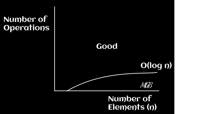
Diagrams
In this case, the runtime increases logarithmically with the size of the input. That is, as n gets very large, the runtime increases, but very slowly. On an `x-y` plane, you can graph the function `f(x) = log(x)`.
Linear Time - O(n)
Linear time, or O(n), describes an algorithm whose runtime increases in direct proportion to the amount of input data. Imagine you're in a line of people and you want to shake hands with each one. The amount of time it will take you to accomplish this task will be proportional to the number of people in the line. If there are 5 people, it will take you 5 times the time it would take if there was only one person. This is the typical behavior of linear time algorithms.
An example of a linear time algorithm is traversing a list or an array of elements, as in the following JavaScript code:
const printColors = (colors) => {
  for (let i = 0; i < colors.length; i++) {
    console.log(colors[i]);
  }
}
Common Usage Examples
Linear time is common in many everyday programming algorithms.
- Every time you traverse a list of items, such as a to-do list.
- When you filter a list of data, you're using linear time algorithms.
- Changing the color of the text of all items in a list on a web page.
- Searching for a specific item in an unordered array.
- They're also common in operations like mapping a list to another one and cloning arrays.
All these examples involve operations that will be performed once for each element in the data set.
Advantages and Disadvantages
Linear time is straightforward and easy to understand. Its main advantage is that it has no specific requirements about the data, unlike logarithmic time which requires the data to be sorted.
However, linear time algorithms can be inefficient for very large data sets. For example, if you have to go through a list of a million elements, the runtime will be proportionately high. If a linear time algorithm takes 1 second to process 1000 elements, it will take approximately 1000 seconds (or about 16 minutes and 40 seconds) to process 1 million elements.
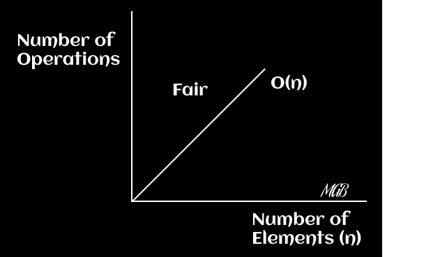
Diagrams
Here, the runtime increases linearly with the size of the input. If the input doubles, the runtime also doubles. On an `x-y` plane, you can plot the function f(x) = x
By mastering the concept of linear time, you will have a better understanding of how to optimize your algorithms for handling large data sets.
💡 Always remember to consider the size of your data when choosing the most efficient algorithm for your task.
Super-Linear Time - O(n log n)
Super-linear time, or O(n log n), describes an algorithm whose runtime is higher than linear but lower than quadratic. This type of time complexity is often found in algorithms that divide the problem into smaller subproblems, solve them independently, and then combine the solutions. To understand it, imagine you're sorting a library of books. If you had to compare each book with every other book (which would be quadratic time), it would take you a long time. But if instead, you could divide the books into smaller groups, sort those groups, and then combine those sorted groups, it would take you less time. This divide and conquer process is more efficient than quadratic time approaches and is the essence of O(n log n) algorithms like Merge Sort.
An example of a super-linear time algorithm is the Merge Sort sorting algorithm:
const mergeSort = (arr) => {
  // If the array's length is less than 2, return the array as is.
  if (arr.length < 2) {
    return arr;
  }

  // Find the middle index of the array.
  const middle = Math.floor(arr.length / 2);

  // Divide the array into two halves around the middle index.
  const left = arr.slice(0, middle);
  const right = arr.slice(middle);

  // Recursively sort both halves and then combine them.
  return merge(mergeSort(left), mergeSort(right));
}

const merge = (left, right) => {
  const sorted = [];

  // Compare the elements of the left and right halves,
  // and place them in the 'sorted' array in the correct order.
  while (left.length && right.length) {
    if (left[0] <= right[0]) {
      sorted.push(left.shift());
    } else {
      sorted.push(right.shift());
    }
  }

  // Combine the 'sorted' array with the remaining elements from the halves.
  return [...sorted, ...left, ...right];
}
Common Usage Examples
Super-linear time algorithms like Merge Sort, Heap Sort, and Quick Sort are widely used in real life to sort large data sets. This is because they are more efficient than quadratic sorting algorithms like Bubble Sort or Insertion Sort, especially for large volumes of data.
Advantages and Disadvantages
The main advantage of super-linear time algorithms is their efficiency in large data sets. This is because the number of comparisons required grows more slowly than the size of the input. However, these algorithms are usually more complex to implement and understand than linear time algorithms. Moreover, some of them, like Merge Sort, require extra memory space to store a temporary copy of the data, which can be costly for very large data sets.
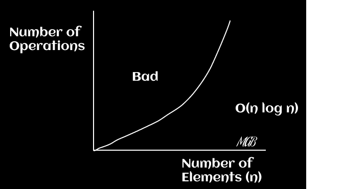
Diagrams
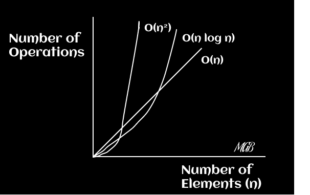
In this case, the execution time is higher than linear but less than polynomial. Typically, algorithms like quick sort fall into this category. You can graph the function f(x) = x * log(x).
Comparisons with the mentioned O(n) and O(n^2)
💡 Tip
When facing coding problems that involve sorting or searching in large data sets, remember that O(n log n) algorithms are a very efficient option. However, it's also important to consider the available memory resources, as some of these algorithms may require extra space. Always remember to weigh the pros and cons based on the specifications of your particular problem. At the end of the day, the correct choice and implementation of algorithms can make a big difference in the performance of your application.
Conclusion
Super-linear time, or O(n log n), is an algorithmic complexity that strikes an effective balance between simplicity and efficiency. Algorithms that have this complexity, like Merge Sort or Quick Sort, are usually an excellent choice for manipulating large data sets, as they increase their execution time more slowly compared to quadratic time algorithms. However, the cost of this efficiency may be higher memory usage and more complex implementation.
Polynomial Time - O(n^2)
Polynomial time, denoted as O(n^k), describes an algorithm whose execution time is proportional to a k power of the size of the input. A common case is O(n^2), which occurs when you need to traverse a list of elements twice - once for each element on the list. Imagine you're at a party and need to shake hands with everyone. For each individual (n), you must greet all the others (n-1). This case, which is quadratic, is just one example of polynomial time, as polynomial time can also refer to complexities such as O(n^3), O(n^4), and so on.
A classic example of a polynomial-time algorithm is Bubble Sort. This sorting algorithm works by traversing the list multiple times and, on each pass, compares each element with the next one and swaps them if they're in the wrong order. This process is repeated until the list is sorted.
const bubbleSort = (arr) => {
  for (let i = 0; i < arr.length; i++) {
    for (let j = 0; j < arr.length - i - 1; j++) {
      if (arr[j] > arr[j + 1]) {
        const temp = arr[j];
        arr[j] = arr[j + 1];
        arr[j + 1] = temp;
      }
    }
  }
  return arr;
}
We have another case like the example of a cubic time algorithm O(n^3) in the context of an e-commerce platform. For example, a function that compares every possible combination of three different products to determine whether they meet certain criteria.
For instance, let's say we are looking for a combination of three products whose total price sums up to a given value (like in the subset-sum problem). The code would look something like this:
function findProductCombination(products, targetPrice) {
  for (let i = 0; i < products.length; i++) {
    for (let j = i + 1; j < products.length; j++) {
      for (let k = j + 1; k < products.length; k++) {
        if (products[i].price + products[j].price + products[k].price === targetPrice) {
          return [products[i], products[j], products[k]];
        }
      }
    }
  }
  return null;
}
The findProductCombination function has a time complexity of O(n^3) as there are three nested loops, each of which can potentially traverse the entirety of the product list. This would be necessary if we were looking for a specific combination of three products that add up to a target price, and the only way to find it would be to go through all the possible combinations of three products.
However, it's important to note that this type of algorithm can be very inefficient for large data sets, as the running time increases with the cube of the size of the product list. In most cases, it would be preferable to find a more efficient solution, especially if you're working with a large product catalog.
Common Use Examples
Polynomial-time algorithms like Bubble Sort, Insertion Sort, and Selection Sort have their place when data sets are small, or the simplicity of the code is an advantage, despite their running time can grow rapidly as the size of the data set increases.
Advantages and Disadvantages
The advantage of polynomial time algorithms lies in their simplicity to understand and implement them. Furthermore, they can be effective for small data sets. However, their main disadvantage is their scalability. As the size of the data set increases, the running time of these algorithms can become prohibitively large.
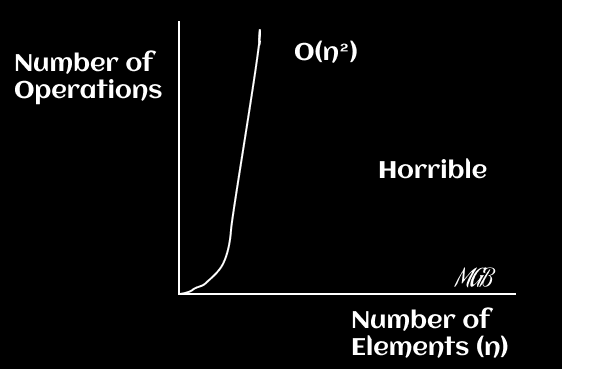
Diagrams
The running time is proportional to the square (or cube, etc.) of the size of the input. You can plot the function f(x) = x^2 for O(n^2) and f(x) = x^3 for O(n^3), etc.
Conclusions
In your analysis of the algorithms and their complexity, it's important to remember that just because an algorithm has a polynomial time complexity (like O(n^2), O(n^3), or O(n^n)) doesn't necessarily make it "bad". It depends on the context and the size of the data you are working with as with many things in programming there is always additional context to consider.
🎗️ For small data sets, a polynomial algorithm may be suitable and even preferable for its simplicity. However, as the size of the data set increases, these algorithms can become very inefficient. Also, bear in mind that although an algorithm may have a worse time complexity in theory, it can have significant improvements in practice due to optimizations from the compiler or the underlying machine we use as a server.
A good developer always seeks a balance between efficiency, readability, and maintainability of code, whereas with the machines we have access to today, readability and maintainability of code are often our top priorities. While it's important to be aware of algorithm efficiency, the clarity and simplicity of the code are also crucial in most of today's web programming environments.
Lastly, in cases where efficiency is crucial and you're dealing with large data sets, you may consider other techniques like more efficient sorting algorithms (like merge sort or quicksort), efficient search algorithms (like binary search), or efficient data structures (like binary search trees).
Exponential Time - O(2^n)
Algorithms with exponential runtime, or O(2^n), have a runtime that grows exponentially with each new element in the input. This means that each additional element can double (or more) the runtime.
A classic example of an exponential time algorithm is the recursive algorithm to calculate Fibonacci numbers. The Fibonacci sequence is a series in which each number is the sum of the two preceding ones, and it starts like this: 1, 1, 2, 3, 5, 8, 13...
The recursive implementation of the calculation of Fibonacci numbers is as follows:
function fibonacci(n) {
  if (n <= 1) {
    return n;
  } else {
    return fibonacci(n - 1) + fibonacci(n - 2);
  }
}
This demonstrates the nature of recursion, where a function calls itself within its own definition.
Common Usage Examples
Although exponential time algorithms are not commonly used in real applications due to their inefficiency, they have a very high educational value. They serve to understand fundamental concepts of recursion and how the efficiency of an algorithm can vary dramatically depending on its implementation.
An example could be a product recommendation system that tries to find all possible combinations of products to maximize the value of the customer's shopping cart without exceeding a certain budget. This is a variant of the brute force knapsack problem, and its direct resolution can involve exponential runtime.
Advantages and Disadvantages
The advantage of exponential time algorithms is their conceptual simplicity, especially when showing how recursive algorithms work. However, their main disadvantage is their inefficiency with larger data sets, where they can cause considerably slow performance or even completely block the program.
Although in its simplest form, the Fibonacci function has exponential time, it can be optimized using techniques such as memoization to reduce the complexity to linear time.
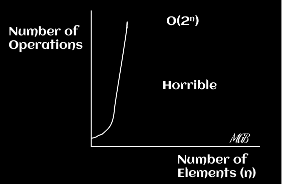
Diagrams
The runtime grows exponentially with each addition to the input. This is one of the least efficient runtimes and can be seen in some search and optimization problems. You can plot the function `f(x) = 2^x`.
Factorial Time - O(n!)
Factorial time algorithms, or O(n!), have a running time that grows extremely fast with each new element in the input. These algorithms are typically the least efficient and their use is limited to very small data sets. The most well-known example of a factorial time algorithm is the Traveling Salesman Problem using brute force strategy.
The Traveling Salesman Problem poses the following question: "Given a list of cities and the distances between each pair of cities, what is the shortest possible route that visits each city exactly once and returns to the origin city?" The brute force strategy to solve this problem involves generating all possible permutations of the cities and identifying the route with the shortest total distance, hence its O(n!) complexity.
// This is pseudocode, not a complete solution for the Traveling Salesman Problem
// The functions generateAllPermutations and calculateTotalDistance are not implemented in this example
const travellingSalesman = (cities) => {
  let shortestDistance = Infinity;
  let shortestPath;

  const permutations = generateAllPermutations(cities);

  permutations.forEach((path) => {
    const distance = calculateTotalDistance(path);

    if (distance < shortestDistance) {
      shortestDistance = distance;
      shortestPath = path;
    }
  });

  return shortestPath;
};
Common Usage Examples
Factorial time algorithms are often used in generating permutations of a dataset. For example, they can be useful in certain fields such as cryptography, where generating all possible keys is necessary for a brute-force attack. Generally, these algorithms are avoided due to their extremely poor performance for large input sizes. However, in certain problems like the Traveling Salesman Problem, brute force (though inefficient) can provide the optimal solution.
Advantages and Disadvantages
Factorial time algorithm can be useful when an optimal solution is needed and the input size is very small. However, for larger data sets, these algorithms are impractical due to their extremely fast factorial growth.
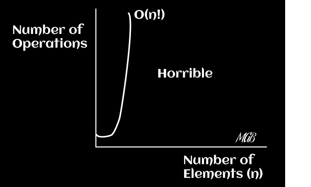
Diagrams
The running time grows extremely fast and is the worst case of complexity. You can plot the function f(x) = x! (factorial of x).
Tips
- Minimize the use of
O(n!)algorithms whenever possible: Although they may be necessary for certain problems, factorial complexity tends to make these algorithms unviable for considerably sized data sets. Always look for more efficient alternatives before resorting to a brute-force approach. - Use optimization strategies: If you find yourself in a situation where an O(n!) algorithm is necessary, consider optimization techniques like pruning, which can eliminate certain branches of computation if they are unlikely to produce an optimal solution.
- Assess the size of your input: Sometimes, an
O(n!)algorithm may be appropriate if you know your data set will always be small. In these cases, simplicity of implementation may be more important than efficiency.
Conclusion
Factorial time algorithms represent a boundary in terms of inefficiency in computing. While they can be useful for certain problems, their real-world application is limited due to their exponential running time growth. Understanding these algorithms serves to reinforce the importance of efficiency in computing and underscores the need to seek more optimized approaches to problem-solving. Learning to identify and handle these cases can be an invaluable skill for any programmer.
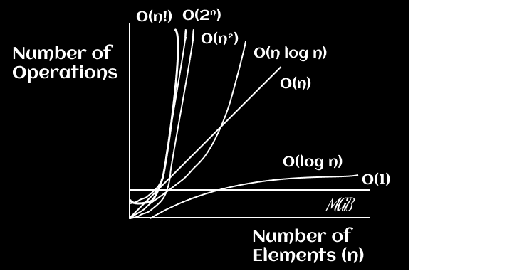
Graphing Big-O Notation
Here is a graph that shows the run times of the aforementioned Big-O and their performance as the size of input data increases.
Constant time is the highest performing runtime and factorial time is the worst performing.
✍️ Final Conclusion
Understanding Big-O notation is crucial for any software developer. It provides a universal language for discussing the performance of algorithms and helps us make more informed decisions when selecting the appropriate data structures and algorithms for our programs. This knowledge will not only help you be a more efficient programmer but will also be invaluable during technical interviews, where you are often expected to justify your choices of algorithms and data structures with reference to their time and space complexity.
🪔 Final Tips
- Practice, practice, practice: As with any concept in computing, the best way to truly understand Big-O notation is by applying it in practice. Try to identify the time and space complexity of algorithms in your own code and in technical interview problems.
- Don't overoptimize: While it's always important to keep efficiency in mind, remember that code readability and maintainability are equally or most important. Not all situations require the most efficient algorithm possible, especially if that makes the code harder to understand and maintain.
- Learn to balance: The choice of the right algorithm or data structure often depends on a balance between time and space. Sometimes, you can achieve a faster runtime by using more memory, or save memory with a slower runtime. Learning to manage this balance is a key skill for any programmer.
I hope this post has provided you with a clear insight into what Big-O notation is and how it is used in programming to analyze the efficiency of algorithms. Your path to becoming an efficient and efficiency-conscious software developer is well on its way, though this is just a smattering of knowledge at the beginning of a long journey.
Thank you for reading this algorithmic complexity series, and I look forward to seeing you in future posts, although it might be on a different topic. Until next time!
References
If you're interested in delving deeper into the topic of time complexity and how it affects the efficiency of your programs, you can refer to the following resources:
- Book: "Introduction to the Design and Analysis of Algorithms" by Anany Levitin.
- Book: "Algorithms Unlocked" by Thomas H. Cormen.
- Book: "Algorithms" by Robert Sedgewick and Kevin Wayne.
- Book: "Algorithm Design Manual" by Steven S. Skiena.
- Book: "Introduction to Algorithms - Fourth Edition" by Thomas H. Cormen, Charles E. Leiserson, Ronald Rivest, Clifford Stein.
- Online Course: Khan Academy: Algorithms
- Online Course: GeekforGeeks: Binary Search
- Online Course: Coursera: Algorithms, Part I
- Online Course: Harvard's CS50: Introduction to Computer Science
- Online Course: Introduction to Algorithms by MIT
- Online Course: Algorithms, Part I by Princeton University
- Online Course: Discrete Optimization by The University of Melbourne
- Video: Logarithms in Computer Science.
- Video: Big O Notations (simple explanation)
- Video: Big O Notations from the "Computer Science Basics" series by HackerRank on YouTube.
- Video: Merge Sort vs. Quick Sort
- Video: Bubble Sort Algorithm
- Video: The Travelling Salesman Problem